Introduction
Intrinsic value is a well defined and often used concept of option pricing theory. It is usually defined as the maximum of zero and the value the option would have if it were exercised immediately. This definition is straightforward to apply to vanilla option with single exercise decision, but its application to more complex options traded in energy markets (e.g. natural gas storage or power tolling) might be confusing. In this blog post we will develop intuition behind the definition of intrinsic value that will help us understand its importance and application to complex options.
Vanilla Options
We start with discussion of vanilla European call option that expires at time T with forward delivering at T as underlying. I.e. the option gives the right to option holder to obtain a unit of commodity at time T for exchange of fixed amount equal to strike K. It is obvious that the option holder would require to pay some money (option premium) to acquire such an option (the payout at time T for the option holder is always bigger than 0). The option pricing theory tries to deduce what price option buyer should pay for this kind of option. Usually the option price depends on time to expiration and properties of the process by which the underlying prices change. However it is possible to find a value that does not depend on the dynamics of prices that bounds option premium from below. One such value we already discussed - it is 0: since the option payout cannot be negative the price of the option should be positive. Can we do better than that?
The more optionality an option provides the more valuable the option is. If we reduce optionality, the value of the option is reduced. So to find lower bound of the option we can consider constraining its optionality. We might require the exercise decision to be made at time \(t = 0\). I.e. at \(t = 0\) the option buyer needs to commit if they receive the unit of commodity at time T for price K. This certainty allows us (the seller) to setup static hedge that replicates payoff at T perfectly:
If the buyer decides to exercise we can enter a forward contract that delivers one unit of the commodity at time T for the fixed price (today's forward rate) \(F_{0}\) (entering such a contract cost nothing at \(t=0\)). At time T we will pay \(F_{0}\) for the commodity and get K from the buyer. Our total PnL is \(K-F_{0}\). Assuming that the interest rate is 0 we would not sell this contract for less than \(F_{0}-K\), otherwise we would incur losses.
If the buyer does not exercise we have nothing to do and we can give away such contract for price 0.
So the option is exercised when \(F_{0}-K>0\). Then the price is \(\left(F_{0}-K\right)_{+}\) which equals to the intrinsic under standard definition.
We see that by restricting an option to the immediate exercise we can create a perfect static hedge that does not depend on the dynamics of the underlying. The value of the restricted option is the intrinsic value of the original option. The intrinsic value is always smaller than the value of the original option.
Hedging and Rolling Intrinsic
By exercising right away and putting static hedge, the option buyer can eliminate risk at the cost of difference between intrinsic value and full price paid for the option. So if \(F_{0}>K\), the buyer will enter short futures position (to sell a unit of the commodity for \(F_{0}\) at time T). At time T the buyer will exercise the option and will pay K for the unit of commodity which s/he then sells for \(F_{0}\), which in total will produce PnL equal \(F_{0}-K\).
Is it possible to improve on this strategy? The simple improvement is called rolling intrinsic strategy:
At time \(t=0\) set up intrinsic strategy (if \(F_{0}>K\) short futures, do nothing otherwise)
If at some future time step \(0 < t < T\) the buyer still doesn't hold short futures position, look at the futures prices. If \(F_{t}>F_{t-1}\) and \(F_{t}>K\) enter short futures position and expect to exercise at expiration.
If have short position (say \(F_{s}\), with \(s < t\) ) and \(F_{t} < F_{s}\) and \(F_{t} < K\) enter long position in \(F_{t}\) to clear \(F_{s}-F_{t}\) and do not exercise at T.
Once at exercise time get \(F_{s}-K\) if still hold short futures position.
In general the rolling intrinsic can be described as follows: we enter each time step t with a possible hedge which is a set of futures that imply exercise decision(s). We check if adjusting the hedge to another exercise decision is profitable - if yes, do that. Notice that this strategy will produce PnL increasing with time. On different price paths PnL paths will be different. Also notice that the rolling intrinsic hedge does not work for American type option, since we used forward contracts with specific delivery time, but American option does not have one.
What about total expected (in risk neutral measure) PnL - how is it related to total option value? As it turns out the expected PnL for rolling intrinsic strategy is a lower bound for the full value of the option. To see this first note that in the risk neutral expectation of any portfolio that trades in forward contracts is equal to 0 (since in risk neutral measure forward rate equals to expected spot.) So the only way why expected PnL for rolling intrinsic can be different than the full value of the option if the rolling intrinsic exercise strategy is different from the optimal exercise strategy. For some options this is true (for example natural gas storage contract - as discussed in the next section), however for vanilla option the rolling intrinsic strategy matches optimal exercise.
Note that even though exercise policy for rolling intrinsic of vanilla option matches optimal exercise on each possible path, the PnL will usually be smaller. Since PnL of vanilla option is always positive we expect that distribution of PnL of rolling intrinsic of vanilla option will be more narrow than PnL produced by exercise at expiration. We show this with an example of option with \(F_{0}=3\), \(\sigma=0.3\), \(T=0.25\), \(K=3.1\) and zero interest rate. We ran the rolling intrinsic policy with 90 steps and ran 100k simulation paths to obtain the following results:
Using Black's formula the value of the option is 0.1366. MC calculated expectation of payoff is 0.1351. MC calculated expectation of PnL of rolling intrinsic is 0.1366. We can see that rolling intrinsic produces value that matches Black's formula. It actually produces better result than regular MC since its distribution is quite more narrow (as we show below).
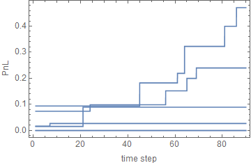
Examples of cumulative PnL produced by rolling intrinsic hedge is presented on the following figure. Notice how the cumulative PnL is always increasing and changes step-wise when exercise strategy changes:
- The standard deviation of unhedged payoff of the option is 0.25. The standard deviation of rolling intrinsic PnL is 0.14, which is quite significantly smaller than unhedged case. The hedging effect of the rolling intrinsic can also be observed on the figure below were we plotted histograms of distributions ungedged and rolling intrinsic PnLs minus value of the option:
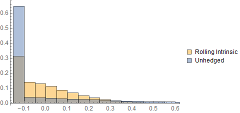
We see that rolling intrinsic hedge has some nice properties: it does work as a hedge, PnL path is always increasing, hedging ratios do not depend on assumptions about dynamics of the process (so the hedge is very robust). However the hedge is not perfect and it does have significant downside.