Summary
The modelling of spot (daily) prices in commodities usually starts with modelling monthly average (forward) prices and then selecting some simple model to describe daily prices within the month relative to the monthly average. The most common model is a simple Geometric Brownian Motion with constant (spot) volatility. In this blog post we show that this approach results in wrong interdependencies (autocorrelation) in spot prices.
We tested two other popular approaches:
- treat daily prices as independent random variables (no autocorrelation)
- assume that the spot prices can be described as a mean-reverting process
We show that we should use the mean reverting process to realistically describe interdependencies of daily prices.
Introduction
The standard approach to modeling daily (spot) prices in commodity markets is to first model the dynamics of the monthly average (forward) and then generate daily prices as offsets from this average. Usually monthly forward contracts and their options have the highest market liquidity so their dynamics can be deduced quite reliably. Since the forward price is equal to the expected average daily price, the expectation for the daily offset should be zero. There are two main approaches to modeling daily prices:
GBM (Geometric Brownian Motion) starting at the level of forward prices.
Independent random log-normal variables with means equal to forward prices.
These approaches ignore spikes, which are usually accounted by the skew in volatility constructions. The main difference between these two approaches is the fact that in the first case the auto-correlation of the daily prices is very high (since each next step is completely defined by the previous). In the second approach the auto-correlation is very low, since every day price is completely independent of previous day prices. This leads to the question we are addressing with this post: Which model better describes the dynamics of daily prices? We will consider the case of power prices and will look into data from ERCOT.
Daily Dynamics in ERCOT
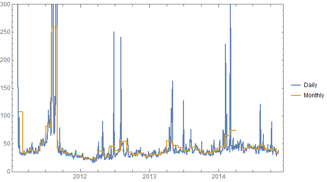
For the analysis we used hourly day-ahead LMP prices from a node in the North Zone of ERCOT. We computed the average of hourly prices over the peak hours (the hour ending 7am through the hour ending 10pm) and skipped weekends and NERC holidays. We also computed the monthly average of these prices:
To find which model best describes the behavior of daily prices we ran the
auto-correlation test (
AutocorrelationTest
in Mathematica) on daily prices within each month. Then we found frequency with
which this test declared prices to be autocorrelated. For the peak ERCOT prices
it was 33%. It is a much bigger number than 5%, which we would get if the prices
were independent (we ran the autocorrelation test with 5% significance level)
and it is much smaller than 95%, which we would get if the prices evolve as GBM.
With this analysis we conclude that neither GBM nor independent variables can realistically describe the interdependence of daily prices. In the next section we will discuss a model that produces more realistic results.
Mean Reverting Daily Prices
Many studies used the mean reverting process to describe the dynamics of spot electricity prices. With discrete time steps the mean reverting process becomes an AR(1) process with an auto-regression coefficient related to the mean reversion:
\[ \begin{align*} d\log p_{t} & =\theta\left(\mu-\log p_{t}\right)dt+\sigma dW_{t}\\ \log p_{d+1}-\log p_{d} & =\theta\mu \Delta t-\theta \Delta t\log p_{d}+\sigma\sqrt{\Delta t}\epsilon_{d}\\ \log p_{d+1} & =\left(1-\theta \Delta t\right)\log p_{d}+\theta\mu \Delta t+\sigma\sqrt{\Delta t}\epsilon_{d} \end{align*} \]
We ran the numerical experiment that showed that if we set the auto-regression coefficient \(\theta \Delta t\) to 0.33 the frequency with which the autocorrelation test declared the prices to be autocorrelated was about 33%, i.e. matched the result for ERCOT daily prices. This suggests that we should use an AR(1) process to model daily prices.
Conclusion
The analysis in this blog post shows that two basic models describing daily prices have very different autocorrelation properties - Geometric Brownian Motion produces price sequences that are perfectly autocorrelated, while treating prices as independent random variables creates price sequences that are not autocorrelated. Usually the actual market prices will fall somewhere in between of these two extremes. The mean reverting model is the simplest model to accommodate this effect.
Please download the Mathematica notebook and data that were used to obtain the results for this blog post. With this notebook you can replicate our calculations or play with a different set of parameters.
Feel free to leave questions or comments below.