Summary
When computing a monthly strip of daily options it is never a good idea to approximate it with a daily option expiring in in the middle of the month (15'th day) as errors in value or implied volatility can be as high as 4%. Instead, it is better to take the daily option that expires after 13.9 days within a month (this halves the errors of the previous method). An even better approach would be to take option that expires depending on how far is the delivery month T - with this method the errors are reduced by a factor of 10 (0.4%). However, this approximation does not work well for deep out of the money options.
Introduction
Daily options are popular contracts in power and natural gas markets. They are European options where underlyings are daily forward contracts for the next day after the exercise. In power markets the forward contract can be peak, off-peak or base load, however in the US only the peak load options are usually liquid. Usually these options are sold in strips (monthly, quarterly, annual). When quoting such a strip the price is given as an average option premium per commodity unit (MWh or MMBtu).
Traders judge if an option is too expensive or too cheap by considering its implied volatility, which is computed using the Black model with a given option premium and price of the underlying. To find the implied volatility, one has to solve the following equation for \(\sigma \):
\[ v_{opt}=B\left(T,F,\sigma\right) \]
where \(v_{opt}\) - option premium, B - Black model, F - price of underlying forward. Similarly, in the case of a monthly strip of daily options one has to solve
\[ \begin{equation} \bar{v}_{opt}=\frac{1}{N}\sum_{i=0}^{N-1}B\left(T + i\Delta t,F,\sigma_i\right) \label{eq:strip} \end{equation} \]
where \(\bar{v}_{opt}\) - average premium of options in the strip, N - number of options in the strip, T - time to the start of the strip (start of the month), \(\Delta t\) - length of one day measured in years, \(\sigma_i\) - daily volatility for the i-th option in the strip.
In practice, to speed up calculations, instead of formula (\ref{eq:strip}) one uses
\[ \begin{equation} \bar{v}_{opt}\thickapprox B\left(T + n\Delta t,F,\sigma_n\right) \label{eq:simplified} \end{equation} \]
where n - some (fixed) day within a strip (say 15'th day if monthly strip is considered). This approximation speeds up calculations quite significantly (factor of 30 for a monthly strip). In this blog post we want to investigate what the best value for n is and what the error introduced by this approximation is.
"Blended" Volatility
Before investigating the approximation described in the Introduction we need to specify how \(\bar{\sigma}_i\) are computed. Forward price dynamics exhibits a term structure of volatility - the farther we are from the delivery period, the lower the volatility ("Samuelson effect"). Therefore the volatility of daily prices should be the highest within the delivery month.
Traders in power markets think about price volatility of daily options in terms of two periods - before the month starts and inside the month. The volatility before the month is described by a monthly option (forward volatility), the market of which is usually more liquid than for daily options. The volatility inside the month is called spot volatility and describes how daily prices behave once we are inside the month. Forward volatilities are usually much lower than spot volatilities. The daily volatilities are then computed by a process that is called "blending":
\[ \begin{equation} \bar{\sigma}_{d}=\sqrt{\frac{\sigma_{F}^{2}T+\sigma_{S}^{2}d\Delta t}{T+d\Delta t}} \label{eq:blending} \end{equation} \]
where \(\bar{\sigma}_{d}\) - daily volatility for day d, \(\sigma_{F}\) - volatility of forward contract that expires at time T, \(\sigma_{S}\) - spot volatility, \(\Delta t\) - time period spanning one day. Traders usually assume that the spot volatility is constant throughout the month.
Examples
For our investigation we will make the following assumptions:
- \(\sigma_F\) is constant and equals 30%
- \(\sigma_S\) is constant and equals 80%
- \(\Delta t\) is one day expressed in years (i.e. 1/365.25)
- a month has 30 days
- we set the interest rate to 0
- we set the forward price of commodity to $50 (per unit)
We are interested in how the approximation (\ref{eq:simplified}) behaves for strikes of different moneyness and different times to the delivery month T. For each case we will present three graphs:
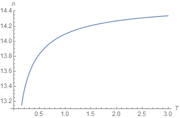
- First we are going to compute at which value of n approximation (\ref{eq:simplified}) yields equality (i.e. at what value of n the option's premium equals the average premium of the strip of daily options.)
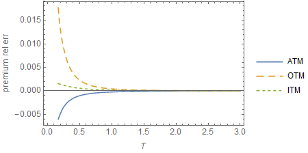
- Then we compute by how much the approximation is different from the exact average premium of daily options for a given n.
- Finally we compute the spot volatility implied by the approximation and compare it to the actual spot volatility \(\sigma_S\).
We will consider only call options (put option results should be similar).
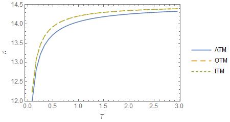
Fixed Moneyness
We consider three cases: at the money \(K = F\), out of the money \(K = 1.2\cdot F\), and in the money \(K = 0.8\cdot F\).
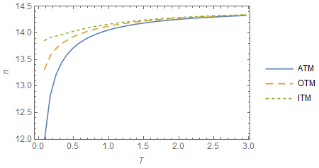
We can see that when we are close to the delivery month (T is small) the optimal value of n decreases. As time to delivery increases n converges to 14.5.
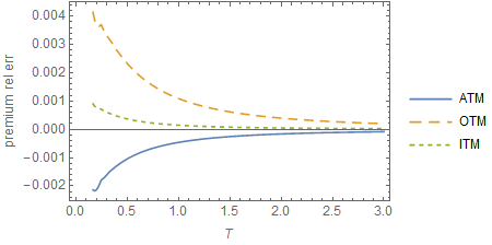
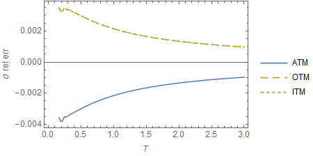
n = 14.5
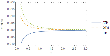
If we use the value of n to which it converges when T is large, the approximation (\ref{eq:simplified}) produces the following errors for value and implied volatility:
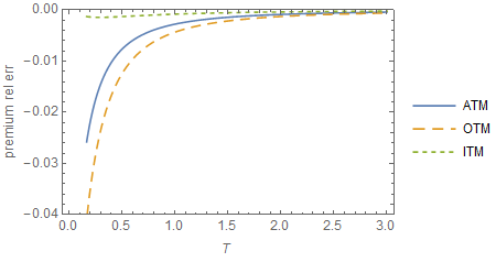
Note that if T is less than about half a year the premium and volatility errors become big and reach almost 4% at T = 2 months.
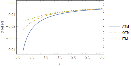
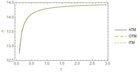
n = 13.9
We can reduce errors observed in the previous section if we pick a smaller value of n = 13.9.
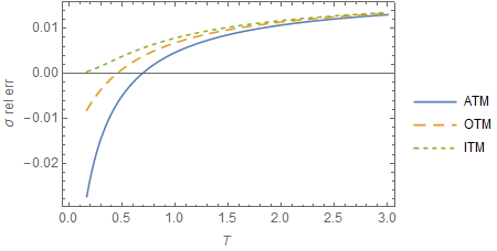
Now both premium and volatility relative errors are within 3% for the full range.
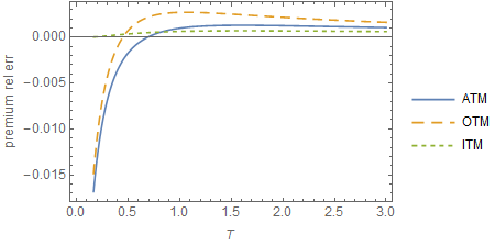
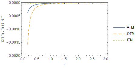
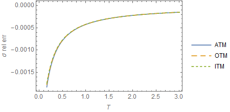
Variable n
We can get a better result if we vary n with T. For this example we set n to be equal to the average of ATM and OTM exact values of n:
With this n we get the following results:
Note that at T > 1 the errors are essentially 0 and they do not increase beyond 2% for small T.
Fixed Reduced Delta
The results in the previous section show how the error becomes very large when T is small. One reason this happens is that when moneyness is fixed, delta becomes very small as T goes to zero. The intuition here is that the underlying distribution width is described by variance \(\sigma^2 T\). When the variance is large even large strikes will fall in a very probable region of the distribution. On the other hand when T is small the variance is small, and even a modest strike can be in a very improbable region of the distribution.
One way to describe moneyness while taking into account the above fact is to use "reduced delta" which is defined as:
\[ D=N\left(\frac{\log\frac{F}{K}}{\sigma\sqrt{T}}\right) \]
To ensure that this "reduced delta" is constant for all T we need to adjust K as follows:
\[ K=Fe^{-d\sqrt{T}} \]
where d is some constant. We select this constant to ensure that \(K/F = 1.2\) at 6 months for the OTM case and \(F/K = 1.2\) at 6 months for the ITM case.
The general shapes of the n curves are similar to the fixed moneyness case, but here ATM and OTM curves are identical.
The error results when n is fixed are similar to the fixed moneyness case (the errors are somewhat smaller, but not significantly), so we will not show them here. However, when we vary n with T (n = average of ATM and OTM exact values of n) we get a much better result:
Note how the relative error is now within 0.4% for the full range of T.
Case: Spot and Forward Volatilities are Close
In previous sections we considered the case when the spot volatility is much larger than the forward volatility (80% vs 30%). But what happens when they are close to each other? (In reality it almost never happens due to the Samuelson Effect.) We ran the above analysis for the case when the spot volatility is just slightly larger than the forward volatility (31% spot vs 30% forward).
Note that the shape of the n curves is similar to the large spot volatility case. However, all moneyness cases are now collapsed into a single curve.
Using n = 14.5, to which it converges for large T, we get the following errors for premium and implied volatility:
The errors are very small (within 0.2% for the full range, for both premium and volatility). If we use 13.9 or variable values for n the errors become even smaller.
Conclusion
Approximating a strip of dailies with the value of a single daily option is an efficient technique for significantly increasing the speed of calculation. However, the time of expiration of the single option needs to be selected carefully. The usual selection with expiration in the middle of the month is never optimal and can produce up to 4% errors for the premium or implied volatility. It is much better to use an option that expires 13.9 days from the beginning of the month, however the errors in this case are still significant - 2%. The best method is to use an expiration date that changes depending on the time to delivery month T. With this method the errors fall below 0.4%.
However, this approach does not work well for deep out of the money options.
You can download the Mathematica notebook that was used to obtain the results for this blog post. With this notebook you can replicate our calculations or play with a different set of parameters.
Feel free to leave questions or comments below.